Distance Analyses
Straight-line (Euclidean) Distance
|
Simple measure (i.e. use a "ruler") | |||||||
|
Query by distance (i.e. select all schools within 1 km of fault line) | |||||||
|
Buffers (fixed distance)
|
|
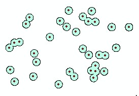
Simple buffer around points
|
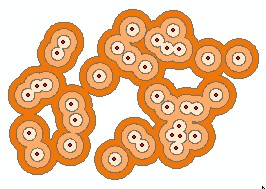
Multi-ring buffer around points.
|
Source: http://www.gis.unbc.ca/courses/geog300/labs/lab12/birdbuff50.jpg
|
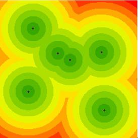
Continuous Euclidean distance (ever-expanding rings of distance) | |
|
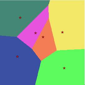
Thiesssen (Voronoi) polygons - Straight-line area allocation (polygon denotes area closest to a point) |
|
Straight-line (Euclidean) distance from points. Rings of the same colour are the same distance from points. |
Straight-line Allocation of area to closest point. This diagram shows Thiessen polygons – the borders of these polygons are equidistant between two points. Therefore the area within a polygon is closest to the point contained within it. Possible examples: 1) Areas that service water wells (i.e. I will go to the nearest well. 2) Determine school catchment areas (maybe too simplistic) |
Network Distance
|
Based on link & turn impedance
| |||||||
|
Shortest / Quickest | |||||||
|
Several Stops (courier/bus route) |
Shortest route over a network.
Source: http://www.storming-robots.com/content/images/direction-shortest-route.gif
|
Area allocation based on network distance (vs. Thiessen polygons) |
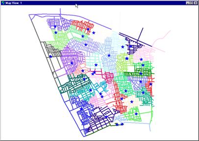
School catchments over a road network.
Source: http://www.fes.uwaterloo.ca/tools/catchmnt.html
|
Emergency Response Areas: determined by both network & surface distance (2 examples): |
|
Base map showing road network. |
Area covered by fire response within 5 minutes |
|
Area covered by fire response within 10 minutes |
Area covered by fire response within 20 minutes |
Four images showing the “area covered” by fire stations for various time intervals.
Note the response time is dependent upon travel over a road network.
Source: http://atlas.scs.carleton.ca/~gis/projects/nemo/ertm.html
Road Travel Time: Coloured areas show travel time it takes to get to downtown Berlin.
Source: http://www.raumplanung.uni-dortmund.de/irpud/pro/berlin/berlin_e.htm
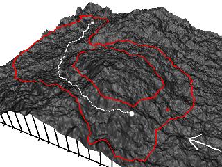
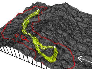
Least-Cost Path
|
Cost (friction) surface |
|
|
“The” cheapest route over a surface. In this case the surface is simply mountainous terrain. |
|
|
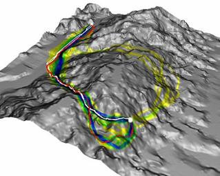
Cheap route options: if a range of cost is allowed, then there is an increase in the routing options. The cheapest route is still shown, but now it is evident that a second (not quite as cheap) route is also available. |
|
|
This is a composite image where several “cheapest routes” are shown. The difference in the routes is dependent on the cost of moving over the landscape. By varying the relative value of the cost variables (steepness, soil types, land use, etc.) we get different routes. |
Source: http://www1.elsevier.com/homepage/sad/cageo/cgvis/ehlschl/paper.htm
Refer to figure 1 and determine the shortest path (route) from the house to the mall for the following:
· As the crow flies
· As the crow mountain bikes
· As the crow pushes a stroller (on sidewalks)
· As the crow drives
![]()

![]()
![]()
|
House |
|
Mall A |


|
|
Figure 1: Distance Analysis Map |

|
Highway |
|
One-Way Street |
|
Cliffs |
![]()
![]()
![]()